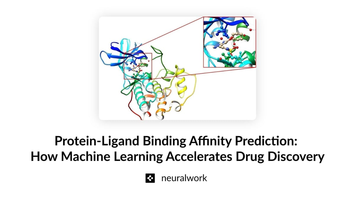
Protein-Ligand Binding Affinity Prediction: How Machine Learning Accelerates Drug Discovery


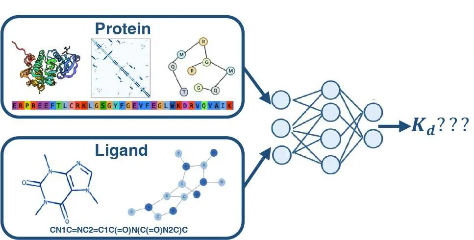
Accurately predicting the binding affinity and configuration between a ligand and its target protein are crucial in drug discovery, which directly affects the drug's effectiveness and selectivity. A high binding affinity is critical not only for the effectiveness of a drug but also for minimizing side effects. When a molecule exhibits low binding affinity to its target protein higher doses of the drug are required to achieve the desired curative effect, which significantly elevates the risk of side effects. A high binding affinity ensures that the drug can modulate the target protein effectively at lower concentrations, reducing the likelihood of adverse reactions and off-target effects. This makes identifying protein-ligand couplings with high binding affinities critical in order to develop safer and more effective curative agents.
Understanding the factors that influence binding affinity through computational analysis helps in the rational optimization of lead compounds. This optimization involves strategically modifying the chemical structure of lead compounds to enhance their interaction with the target protein, and thus their effectiveness and selectivity. This iterative process, guided by binding affinity predictions, allows for efficient exploration of the chemical space to identify optimal drug candidates. Moreover, analyzing the predicted binding pose within the protein's binding site provides mechanistic insights into the molecular interactions governing affinity, enabling the design of drugs.
How does machine learning comes into play in these tasks? Traditionally, identifying potential drug candidates involves synthesizing compounds and experimentally testing their binding affinity to target proteins — a laborious and time-consuming effort. This is why computational methods like molecular docking and quantitative structure-activity relationship (QSAR) models have quickly rose to popularity to estimate these interactions. However, these approaches often struggle with accuracy and scalability, limiting their effectiveness in large-scale drug screening efforts. Leveraging and learning from vast amounts of data, machine learning methods are attractive candidates to solve this problem as they can infer previously obscured patterns and relationships, revealing hidden insights that may be difficult to discern through conventional and semi-conventional experimental approaches alone.
In this blog post, we will talk about the fundamentals of protein-ligand binding affinity prediction and develop a tool for the early stages of the drug discovery process to make it easier to predict potential drug candidates accurately. For this tutorial, we will use the open-source BELKA dataset and train a Random Forest model, which has demonstrated significant promise in addressing these challenges due to its ability to handle high-dimensional data and model complex non-linear relationships. This ensemble learning method, which builds and combines multiple decision trees, effectively capture the intricate interactions between proteins and ligands.
Dataset
In this blog post, we will be using Leash Biosciences' The Big Encoded Library for Chemical Assessment (BELKA) (link) dataset. This large dataset contains binding affinity data for approximately 133 million small molecules tested against three protein targets using DNA-encoded chemical library (DEL) technology. The targets proteins in this dataset are carefully selected and are as follows:
- Human Serum Albumin (HSA): A major protein in blood plasma that transports various substances, including drugs, throughout the body.
- Bromodomain-containing protein 4 (BRD4): A protein that regulates gene expression and is implicated in cancer and inflammatory diseases.
- Soluble Epoxide Hydrolase (sEH): An enzyme involved in the metabolism of fatty acids, with potential therapeutic implications in cardiovascular and inflammatory diseases.
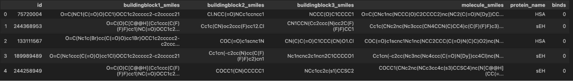
Dataset Schema
- buildingblock1_smiles, buildingblock2_smiles, buildingblock3_smiles: Smaller chemical entities or fragments used as the starting materials in the synthesis of larger molecules. Each building block represents a part of the final compound.
- smiles_molecule: Final synthesized compound that results from combining the building blocks. It is the complete chemical entity that may interact with the protein target.
- protein_name: One of the 3 target proteins.
- binds: Value representing whether the molecule can successively bind to the target protein.
Building blocks and compound molecules in the BELKA dataset are given in SMILES format - Simplified Molecular Input Line Entry System. This notation allows a user to represent a chemical structure with short ASCII strings such that they can be processed by computers.
Data Exploration and Visualization
Let's start by loading and sampling a subset of the BELKA dataset. Before we start, make sure to head to Kaggle and download the training dataset of BELKA. Note that the training and test datasets of BELKA are provided in csv, as well as compressed parquet formats. For this tutorial, we will use the parquet version (train.parquet, which is 3.76 GB) and leverage the duckdb Python library to subsample the dataset with SQL-like queries. Let's start by installing the duckdb, pandas and scikit-learn libraries to load and transform the dataset:
pip install duckdb
pip import pandas
pip install scikit-learn
We will start by subsampling 100,000 rows of data that contains 50,000 binding and 50,000 non-binding samples. To do this, we will use the duckdb library to query the previously downloaded train.parquet file and load the subsampled data into a pandas dataframe.
import duckdb

# edit this to point to the training dataset on your local
train_path = '<PATH_TO_DATA>/train.parquet'
con = duckdb.connect()

df = con.query(f"""
    (SELECT *
    FROM parquet_scan('{train_path}')
    WHERE binds = 0
    ORDER BY random()
    LIMIT 50000)
    UNION ALL
    (SELECT *
    FROM parquet_scan('{train_path}')
    WHERE binds = 1
    ORDER BY random()
    LIMIT 50000)"""
).df()

con.close()

# print out the first 5 rows of data
print(df.head())
Now that we have loaded and subsampled the dataset, one of the best ways to understand the data we are working with is visualization. Luckily for us, there are multiple chemical toolbox python libraries that makes visualizing chemical structures in 2D and 3D formats very easy. Let's go ahead and install the RDKit and Py3DMol libraries we will use:
pip install rdkit
pip install py3Dmol
Next, we will define a function that will take in a molecule in SMILES format (e.g. O=C(Nc1c(Cl)cccc1C(=O)O)OCC1c2ccccc2-c2ccccc21), convert it to molecular representation and visualize it in 2D.
from rdkit import Chem
from rdkit.Chem import Draw
from rdkit.Chem import AllChem

def visualize_mol(smiles, size=(360, 360)):
    # convert the SMILES string to a molecule object
    mol = Chem.MolFromSmiles(smiles)

    # draw and display the molecule
    Draw.MolToImage(first_molecule, size=size)
    return
Let's go ahead and visualize the building blocks as well as the compound molecule of the first data sample in the BELKA dataset.
visualize_mol(df['buildingblock1_smiles'].iloc[0])
visualize_mol(df['buildingblock2_smiles'].iloc[0])
visualize_mol(df['buildingblock3_smiles'].iloc[0])

# visualize the compound molecule
visualize_mol(df['molecule_smiles'].iloc[0])
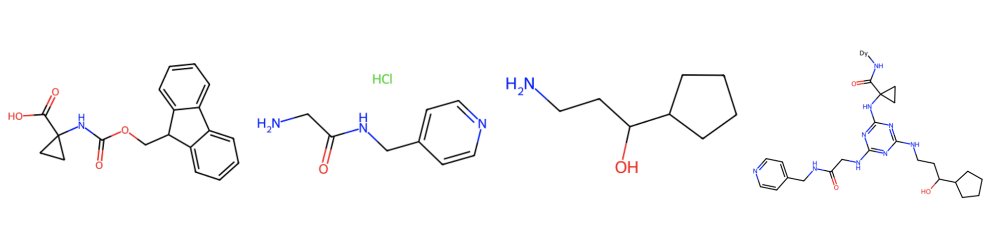
The compound molecule includes all three building blocksand is the complete chemical entity that can interact with the protein target. To take a better look at the compound molecule, we can alternatively use the Py3DMol library, which supports 3D visualizations.
import py3Dmol

def visualize_molecule_3dmol(smiles):
   mol = Chem.MolFromSmiles(smiles)
   if mol:
       viewer = py3Dmol.view()
       viewer.addModel(Chem.MolToMolBlock(mol), 'mol')
       viewer.setStyle({'stick': {}})
       viewer.zoomTo()
       viewer.show()


visualize_molecule_3dmol(df['buildingblock1_smiles'][1])
visualize_molecule_3dmol(df['buildingblock2_smiles'][1])
visualize_molecule_3dmol(df['buildingblock3_smiles'][1])
visualize_molecule_3dmol(df['molecule_smiles'][1])
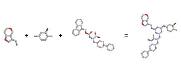
SMILES strings often represent molecules with implicit hydrogens, meaning the hydrogen atoms are not explicitly listed but are understood to be there. For accurate 3D modeling, these implicit hydrogens need to be made explicit to complete the molecular structure. Let's go ahead and perform a more accurate 3D visualization this time. For more details and tips, refer to the RDKit Cookbook.
# convert the SMILES string to an RDKit molecule object
mol = Chem.MolFromSmiles(df['molecule_smiles'].iloc[0])

# add hydrogen atoms to the molecule
mol = Chem.AddHs(mol)

# embed the molecule in 3D space
mol = AllChem.EmbedMolecule(mol)

# visualize the molecule in 3D using Py3Dmol
view = py3Dmol.view(width=800, height=600)
mol = Chem.MolToPDBBlock(mol)
view.addModel(mol, 'pdb')
view.setStyle({'stick': {}})
view.zoomTo()
view.show()
Preprocessing and Feature Extraction
Given a dataset of inputs and corresponding outputs, machine learning models try to learn the parameters of a function that accurately approximates this mapping such that it can be generalized to previously unseen inputs. While the function we are trying to learn the parameters of depends on the machine learning model or network architecture we choose, it always requires the input data to be in a format that is expressive, numerical and meaningful. Training a machine learning model for predicting drug binding affinities is no different as it requires features that can capture the complex details of molecular interactions.
To train a model on the BELKA dataset, we will extract Extended Connectivity Fingerprints of the candidate molecules and one-hot encode target proteins, such that each of the 3 target proteins in the dataset will be assigned a unique class id. While we simply apply one-hot encoding to proteins due to the low and fixed number of target proteins in the dataset, working with datasets that are more diverse would require more meaningful and rich representations such as Protein2Vec.
Extended Connectivity Fingerprints (ECFPs):
ECFPs are a type of molecular fingerprint that captures the structure of a molecule. They are widely used in cheminformatics to represent molecules numerically. Advantages of ECFPs compared to other chemical representations such as Morgan Fingerprints and MACCS keys are as follows:
- Rich Structural Representation: ECFPs encode detailed information about molecular substructures, such as rings, chains, and functional groups, which are critical for identifying how molecules interact with proteins. Unlike Morgan fingerprints and MACCS keys, ECFP is optimized for compatibility with ML algorithms.
- MACCS keys use a fixed set of 166 predefined structural features, which can limit their ability to capture the full complexity of molecular interactions.
- Morgan fingerprints lack the detailed structural representation and machine learning compatibility that ECFP offers, resulting in lower predictive accuracy for protein-ligand binding affinity.
- Scalability: ECFPs can handle large molecular datasets efficiently, providing a scalable solution for high-throughput screening in drug discovery.
- Proven Effectiveness: ECFPs have been extensively validated in various studies for their ability to predict molecular properties and bioactivity.
- Robustness to Isomers: They account for the presence and connectivity of atoms, making them robust in distinguishing between isomers which may have different biological activities.
To convert SMILES strings (a textual representation of the molecule) into ECFPs, we will use the RDKit library and define a wrapper function to apply this transformation to all data rows. The resulting fingerprints are bit vectors that capture the presence or absence of particular substructures in the molecule.
Morgan fingerprints is a general method for encoding molecular structures into bit vectors and Extended Connectivity Fingerprints (ECFPs) are a specific type of Morgan fingerprint with predefined settings (e.g. radius=2 for ECFP4) which are optimized for capturing molecular substructures. By using 'AllChem.GetMorganFingerprintAsBitVect(molecule, radius, nBits=bits)', we can generate ECFPs with a more detailed and consistent representation.
def generate_ecfp(molecule, radius=2, bits=2048):
   if molecule is None:
       return None
   return list(AllChem.GetMorganFingerprintAsBitVect(molecule, radius, nBits=bits))


# convert SMILES data to Morgan Fingerprints
df_test['molecule'] = df_test['molecule_smiles'].apply(Chem.MolFromSmiles)
df_test['ecfp'] = df_test['molecule'].apply(generate_ecfp)
The next step is to one-hot encode the protein names, such that each of the 3 target protein names is treated as a category. One-hot encoding is a straightforward method that effectively transforms categorical variables into a binary matrix, allowing to interpret protein identities numerically. To do this, we will use the scikit-learn library and create 3 new, binary dataframe columns where each column corresponds to a unique protein name.
import pandas as pd
from sklearn.preprocessing import OneHotEncoder


onehot_encoder = OneHotEncoder(sparse_output=False)
onehot_encoder.fit(pd.Series(protein_names).values.reshape(-1, 1))

protein_onehot = onehot_encoder.transform(df_test['protein_name'].values.reshape(-1, 1))
Once we have extracted the Extended Connectivity Fingerprints and one-hot encoded the protein_name column of the dataset, we need to combine these to form a single feature vector for each data sample. Additionally, we need to separate the binds values to create a target output vector for model training.
from sklearn.model_selection import train_test_split

# combine fingerprint and one-hot encoded protein features
X = [ecfp + list(protein) for ecfp, protein in zip(df['ecfp'].tolist(), protein_onehot.tolist())]

# target binding values to we would like to predict
y = df['binds'].tolist()

# split model input and outputs to train and test sets
X_train, X_test, y_train, y_test = train_test_split(X, y, test_size=0.2, random_state=42)
Predictive Modeling with Random Forest
We can now move onto predictive model training. For this tutorial, we will train a Random Forest model, and show how to optimize model performance and robustness via hyperparameter search and cross-validation.
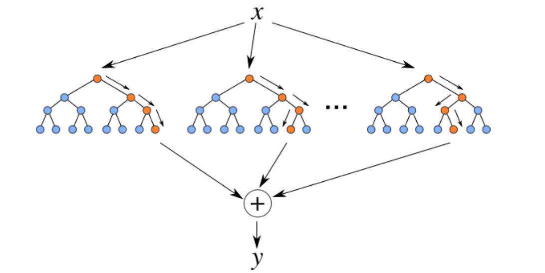
Random Forest is an ensemble machine learning method that constructs multiple decision trees during training. Each tree is built using a bootstrapped sample of the data and a random subset of features for each split, ensuring diversity among the trees. The final prediction is made by aggregating the predictions from all trees, which helps reduce overfitting and improve generalization.
Hyperparameter Tuning with Randomized Search
Hyperparameters of any statistical model can massively impact the model's performance during training and testing. For Random Forest, such hyperparameters include the number of trees in the forest (n_estimators), the maximum depth of each tree (max_depth), the minimum number of samples required to split a node (min_samples_split), the minimum number of samples required to be at a leaf node (min_samples_leaf), the number of features to consider when looking for the best split (max_features), and whether bootstrap samples are used when building trees (bootstrap). While we can an educated guess about some of these, hyperparameter optimization is generally a good practice to ensure optimal results. In this tutorial, we perform hyperparameter optimization using Randomized Search Cross-Validation such that the models are trained and tested on various different data splits to ensure generalization capabilities. This approach involves randomly sampling from a predefined hyperparameter space and evaluating the model using cross-validation to identify the best set of hyperparameters.
from sklearn.model_selection import RandomizedSearchCV
from sklearn.ensemble import RandomForestClassifier


params = {
   'n_estimators': [100, 200, 300],
   'max_depth': [None, 10, 20, 30],
   'min_samples_split': [2, 5, 10],
   'min_samples_leaf': [1, 2, 4, 6],
   'max_features': ['sqrt'],
   'bootstrap': [True, False]
}
random_search = RandomizedSearchCV(
    estimator=RandomForestClassifier(random_state=42),
    param_distributions=params,
    n_iter=100,
    cv=4,
    n_jobs=-1,
    verbose=2,
    scoring='average_precision',
    random_state=42
)

# fitting 5 folds for each of 432 candidates, a total of 2160 fits
random_search.fit(X_train, y_train)

# retrieve the best model
best_model = random_search.best_estimator_
Model Evaluation
After performing hyperparameter search and identifying the highest performing Random Forest model, we evaluate this model's performance on the test set by predicting the binding affinities and computing an error term based on ground truth binding affinities:
y_pred_probs = best_model.predict_proba(X_test)[:, 1]
The model's predictive performance is assessed using the Mean Squared Error (MSE) and feature importance analysis to understand the contribution of each feature to the predictions. MSE is a widely used metric for the binding affinity prediction task as binding affinity is typically measured and reported by the equilibrium dissociation constant ($K_D$), which is used to evaluate and rank order strengths of biomolecular interactions. The smaller the $K_D$ value, the greater the binding affinity of the ligand for its target. However, the BELKA dataset contains binary (0/1) binding affinity values and therefore we report additional metrics such as precision, average precision and cross validation score.
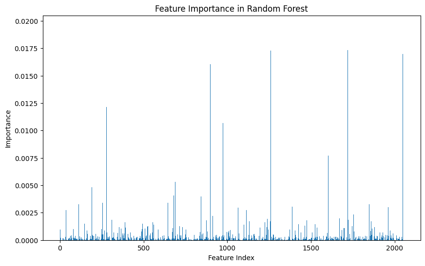
The feature importance analysis of our trained Random Forest model reveals a concentrated influence of a few key features on the model's predictive power. This insight points to opportunities for feature selection or engineering to streamline the model and potentially enhance its performance and interpretability.
As mentioned earlier, the binding affinities in the BELKA dataset are binary. Hence, binary classification metrics such as precision, recall and average precision make more sense to measure to model's performance. The main difference between precision and average precision is precision assigns predictions to binary values (0/1) based on a single threshold value, usually 0.5, whereas average precision requires performing the same assignment based on multiple threshold values (e.g. 0.3, 0.5, 0.7) and taking the average of per threshold precision values. To demonstrate this, let's cross validate our trained model on various subsets of the training data using average precision as our target metric.
from sklearn.model_selection import cross_val_score


# Perform cross-validation
cv_scores = cross_val_score(best_model, X_train, y_train, cv=5, scoring='average_precision')
print(f"Cross-Validation Scores: {cv_scores}")
print(f"Mean CV Score: {np.mean(cv_scores)}")

Cross-Validation Scores:
[0.96097772 0.96540852 0.95846032 0.96396381 0.96033713]
Mean CV Score: 0.9618294985973149
Impressive but not very meaningful results as we have tested our model on the same data it was trained on. Let's go ahead and test our model on the test set, and compute the confusion matrix and receiver operating characteristic curve (ROC). For these analysis, we will set the binary classification threshold to 0.5.
from sklearn.metrics import confusion_matrix, ConfusionMatrixDisplay

threshold = 0.5
y_pred = (y_pred_probs >= threshold).astype(int)
cm = confusion_matrix(y_test, y_pred)

disp = ConfusionMatrixDisplay(confusion_matrix=cm, display_labels=best_model.classes_)
disp.plot(cmap=plt.cm.Blues)
plt.title('Confusion Matrix')
plt.show()
from sklearn.metrics import roc_curve, auc

# Compute ROC curve and ROC area
fpr, tpr, _ = roc_curve(y_test, y_pred_probs)
roc_auc = auc(fpr, tpr)

# Plot ROC curve
plt.figure(figsize=(8, 6))
plt.plot(fpr, tpr, color='darkorange', lw=2, label=f'ROC curve (area = {roc_auc:.2f})')
plt.plot([0, 1], [0, 1], color='navy', lw=2, linestyle='--')
plt.xlim([0.0, 1.0])
plt.ylim([0.0, 1.05])
plt.xlabel('False Positive Rate')
plt.ylabel('True Positive Rate')
plt.title('Receiver Operating Characteristic (ROC) Curve')
plt.legend(loc="lower right")
plt.show()
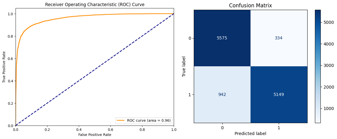
As seen in the figures, our trained model performs reasonably well on the previously unseen test dataset, achieving a precision score of 0.939, a recall score of 0.845 and an F1 score of 0.889. While there are 942 binding samples falsely labeled as non-binding, the vast majority of samples predicted to be binding are true positives. A high precision and relatively lower recall can be interpreted as the model can be further improved upon to discriminate between non-binding and binding classes, yet it is highly reliable when it labels samples as binding.
Further Improvements
In this blog post, we talked about the protein-ligan binding affinity prediction problem and its significance for drug discovery. We introduced chemical toolset Python libraries and demonstrated how we can represent and train machine learning models such as Random Forest on chemical data. We also talked about how to validate the performance of such models and what metrics can be used. While we trained a model that performs reasonably well, there are many ways and methods to improve the model performance. A non-exhaustive list of potential improvements and suggestions are as follows:
- Feature Selection:
- The feature importance plot highlights several features with negligible contributions. Removing these features can simplify the model and potentially improve its performance by reducing noise and overfitting.
- Investigate potential interactions or combinations of less important features that might collectively have a stronger impact on predictions.
- Hyperparameter Tuning:
- Revisit and refine hyperparameters, especially focusing on parameters that control the model's complexity, such as tree depth, minimum samples split, and the number of trees.
- Employ cross-validation techniques like k-fold cross-validation to ensure that the model's performance generalizes well to unseen data.
- Model Selection:
Experiment with other classical ML models such as K-NN or more complex architectures such as Graph Neural Networks, Transformers, which are good candidates to learn from chemical data. Deep learning approaches enable iterative training, hence making it possible to train models on much larger datasets. - Data Representation:
Experiment with different molecular and protein representations such as different chemical fingerprints or learned chemical embedding models such as protein2vec and Mol2vec. Richer representations that can capture structural and semantic information that might not be evident in simpler molecular descriptors would potentially enhance the model's ability to learn from subtle patterns.