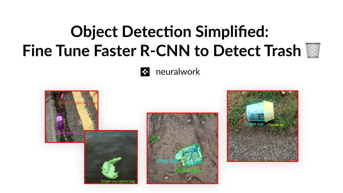
Object Detection Simplified: Fine Tune Faster R-CNN to Detect Trash

Introduction
Trash and marine debris pollution pose significant environmental challenges, that impact ecosystems, wildlife, and human health. Detecting and classifying trash in diverse and complex environments is a significant challenge. The manual process of identifying and cataloging trash is not only labor-intensive and time-consuming but also prone to errors and inconsistencies. Traditional methods fall short in providing the scalability and precision needed for effective environmental monitoring and waste management especially in areas that are difficult to access, such as remote beaches, dense urban settings, and ocean surfaces.
On the other hand, automated systems that leverage advanced machine learning algorithms for trash classification and detection offer potential to drastically improve the efficiency and accuracy, which are crucial for environmental monitoring and waste management. These systems can inform and enhance conservation strategies, ultimately contributing to more sustainable environmental practices.
The objective of this project and blog post is to develop a reliable object detection model to accurately detect different categories of trash. To this end, we will be leveraging ResNet50 as a feature extractor, which will be integrated with Faster R-CNN framework for object detection. ResNet50 is employed to extract rich, high-dimensional features from the input images, whereas Faster R-CNN utilizes these features for precise localization and classification of trash objects. To enhance the model's generalizability and reliability, we will implement a 5-fold cross-validation strategy and evaluate the model's performance across diverse data splits. In summary, our goal is to create a model that can:
-Accurately detect various types of trash: capable of identifying different forms of waste, including plastic, glass, metal, and organic materials, in a wide range of environments.
- Enhance efficiency in environmental monitoring: automating the detection process allowing for more frequent and comprehensive monitoring.
- Support Conservation and Waste Management Efforts: providing reliable data on the distribution and composition of trash.
This project is created as a part of voluntary involvement with Eyesea, a nonprofit organization commited to mapping global pollution and maritime hazards. Eyesea's approach involves crowdsourcing data through geotagged images, creating a visual representation of marine debris and hazards. You may consider to contribute with the same local trash to here.
Table of Contents
TACO Dataset
TACO (Trash Annotations in Context) is an open-source image dataset that captures waste in various environments, from tropical beaches to urban streets. It consists of manually labeled images with bounding box annotations and segmentation maps in COCO format to support training and evaluating object detection and segmentation models. While the official dataset comprises 1,500 images with 4,784 annotations, TACO is a growing project, aiming to expand its collection to 10,000 annotated images. Feel free to contribute with your local trash from here.
Why TACO?
- Data Diversity: images from diverse environments such urban areas, natural settings, and coastal regions for robust and generalizable detection.
- Rich Annotations: rich and granular bounding boxes and segmentation labels.
- Multiple Categories: covers 60 distinct types of litter, 28 distinct supercategory.
To get started with coding, head over to TACO's Github repository and follow the instructions to download the dataset to you local.
Data Exploration
Let's start by importing essential libraries for data manipulation (pandas), visualization (matplotlib, seaborn), image handling (Pillow). If haven't done so, start by installing the dependencies we will need for exploration and modeling:
pip install pandas
pip install matplotlib
pip install seaborn
pip install Pillow

pip install scikit-learn
pip install torch
pip install torchvision
# import dependencies for data exploration
from collections import Counter

import pandas as pd
from PIL import Image
import matplotlib.pyplot as plt
import matplotlib.patches as patches
import seaborn as sns
Next, we will load the metadata and print the first few rows to take a look at the data structure.
# load the metadata
metadata_df = pd.read_csv('meta_df.csv')
print(metadata_df.head())
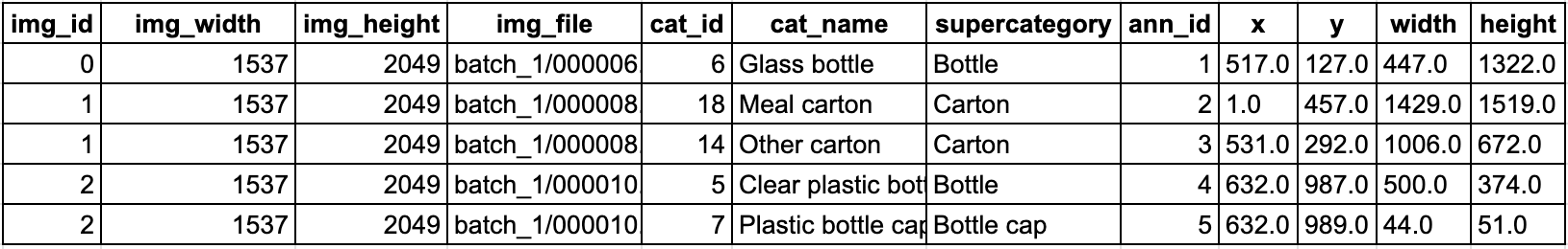
The dataset is in COCO format and contains image ID, annotation ID, image dimensions, file paths, category IDs, and bounding box coordinates (x, y, width, height). Note that there can be multiple bounding box annotations for the same image. Let's go ahead and print out some relevant statistics:
print(f"Total image count: {metadata_df['img_file'].nunique()}")
print(f"Total annotation count: {len(metadata_df)}")
print(f"Unique supercategory count: {metadata_df['supercategory'].nunique()}")
>>> Total image count: 1500
>>> Total annotation count: 4784
>>> Unique supercategory count: 28
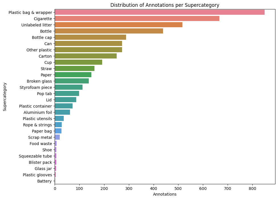
TACO dataset is relatively small with 28 supercategories. Hence, it is useful to plot the distribution of annotations per supercategory in order to decide whether there is a sufficient number of samples for each supercategory. Our plot shows that "Plastic bag & wrapper" and "Cigarette" have the highest annotation counts:
supercategory_counts = metadata_df['supercategory'].value_counts()
plt.figure(figsize=(10, 8))
sns.barplot(y=supercategory_counts.index, x=supercategory_counts.values, palette='husl')
plt.title('Distribution of Annotations per Supercategory')
plt.xlabel('Annotations')
plt.ylabel('Supercategory')
plt.show()
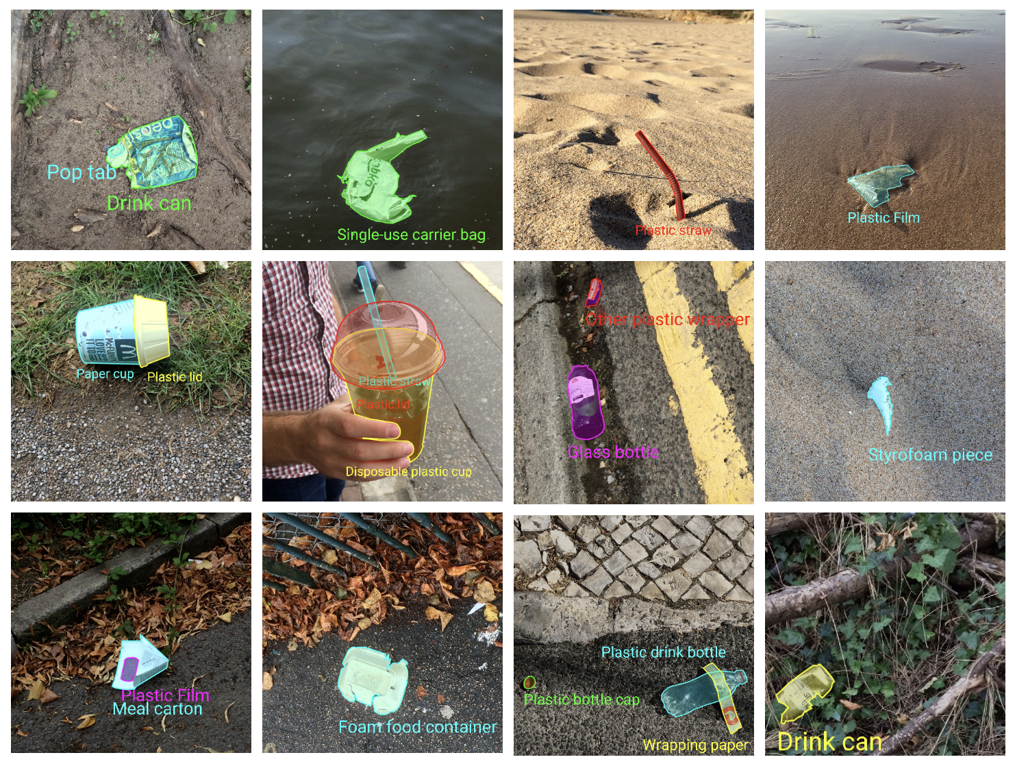
Finally, let's load and display sample images with bounding boxes and category labels to make sure the annotations are reliable:
# visualize some images with bounding boxes
def show_image_with_bboxes(image_path, boxes, labels):
    image = Image.open(image_path)
    fig, ax = plt.subplots(1, figsize=(4, 4))
    ax.imshow(image)
    for box, label in zip(boxes, labels):
        x1, y1, w, h = box
        rect = patches.Rectangle((x1, y1), w, h, linewidth=2, edgecolor='r', facecolor='none')
        ax.add_patch(rect)
        plt.text(x1, y1, label, color='white', fontsize=6, backgroundcolor='red')
    plt.show()

example_images = metadata_df['full_path'].unique()[:6]

for img_path in example_images:
    img_data = metadata_df[metadata_df['full_path'] == img_path]
    boxes = img_data[['x', 'y', 'width', 'height']].values
    labels = img_data['supercategory'].values
    show_image_with_bboxes(img_path, boxes, labels)

With the dataset prepared and visualized, the next step is to define the model architecture, preprocess the data and move onto model training.
Model Architecture
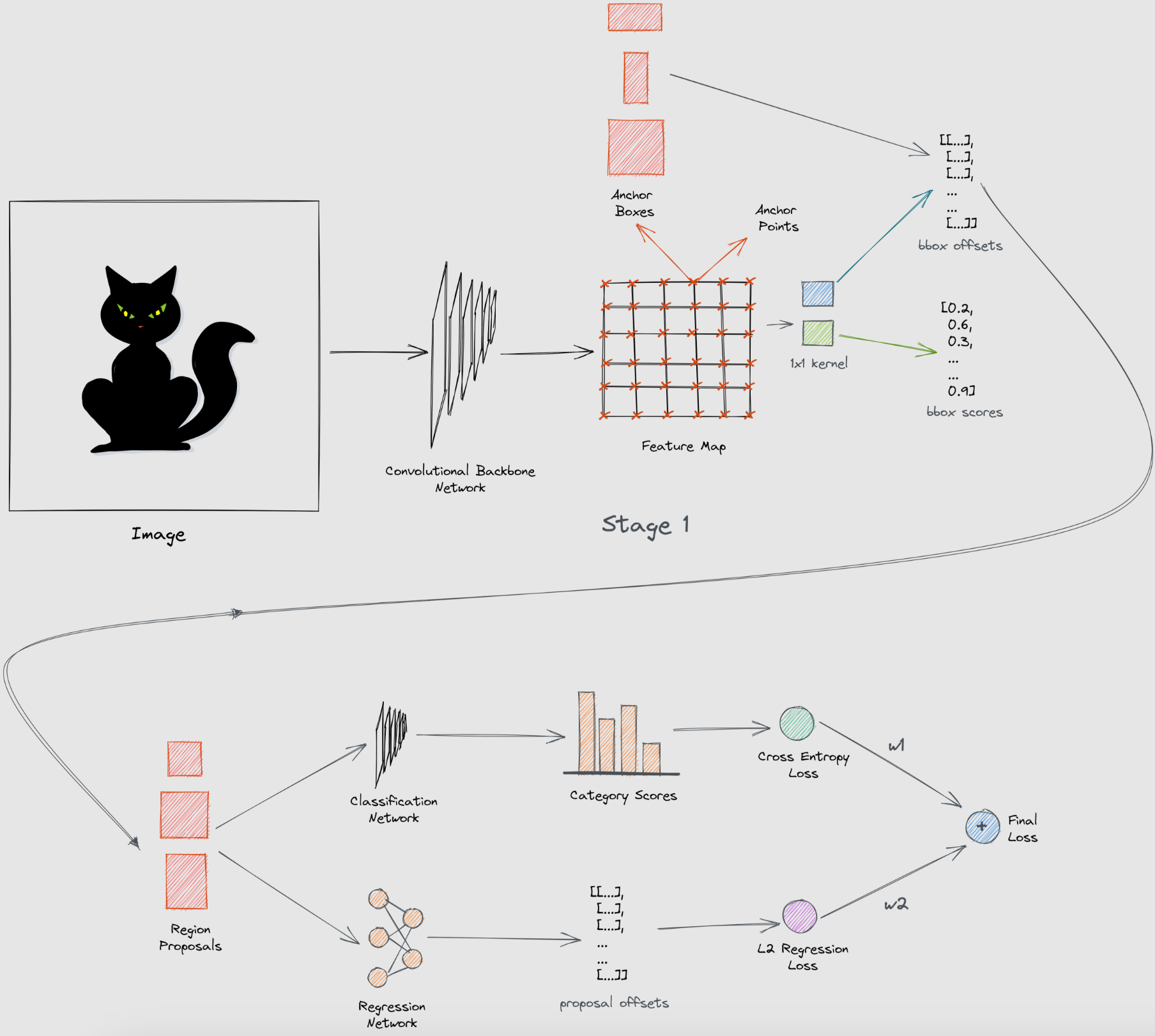
In this project, we will be training a Faster R-CNN model with a ResNet-50 backbone for object detection. Faster R-CNN is a widely used object detection model that combines a region proposal network (RPN) with classification and regression networks, providing efficient and accurate object detection capabilities. ResNet-50 serves as Faster R-CNN's feature extractor in this setup, enabling the extraction of robust deep features from the input images: Input Image -> [ResNet] -> Feature Map. The Region Proposal Network (RPN) scans the feature map with a sliding window, proposing anchors that likely contain objects: Feature Map -> [RPN] -> Region Proposals. Finally, the output region proposals are fed through both a regression network and a classification network to output bounding boxes and classification labels.
While there are other models such as YOLO (You Only Look Once) or SSD (Single Shot MultiBox Detector) that are capable of real-time object detection, we choose Faster R-CNN as our target model as it is known to perform better, especially for detecting smaller objects, which are prevalent in the TACO dataset.
Fine-tuning Faster R-CNN
Custom Model Class
While the TACO dataset features high quality annotations, it is too small to train a Faster R-CNN model from scratch. To make this task a bit easier, we will start from a pre-trained model that was trained on the COCO V1 dataset. In order to finetune this pre-trained model, we will start by defining a custom class FasterRCNNWithCustomClassifier:
import torch
import torch.nn as nn


class FasterRCNNWithCustomClassifier(nn.Module):
    def __init__(self, num_detection_classes, num_classification_classes):
        super(FasterRCNNWithCustomClassifier, self).__init__()
        # load pre-trained model
        self.faster_rcnn = torchvision.models.detection.fasterrcnn_resnet50_fpn_v2(weights="DEFAULT")

        # update the regression network to handle the new detection classes
        in_features = self.faster_rcnn.roi_heads.box_predictor.cls_score.in_features
        self.faster_rcnn.roi_heads.box_predictor = torchvision.models.detection.faster_rcnn.FastRCNNPredictor(in_features, num_detection_classes)

        # overwrite the classification network
        self.out_channels = self.faster_rcnn.backbone.out_channels

        self.classification_head = nn.Sequential(
            nn.AdaptiveAvgPool2d((1, 1)),
            nn.Flatten(),
            nn.Linear(self.out_channels, 512),
            nn.ReLU(),
            nn.Dropout(0.5),
            nn.Linear(512, num_classification_classes)

    def forward(self, images, targets=None):
        if self.training and targets is not None:
            # compute loss terms
            detection_losses = self.faster_rcnn(images, targets)
        else:
            # only return detection results
            detection_results = self.faster_rcnn(images)

        features = [self.faster_rcnn.backbone(image.unsqueeze(0)) for image in images]
        last_feature_maps = [list(f.values())[-1] for f in features]
        last_feature_map = torch.cat(last_feature_maps, dim=0)

        classification_output = self.classification_head(last_feature_map)

        if self.training and targets is not None:
            return detection_losses, classification_output
        else:
            return detection_results, classification_output
The FasterRCNNWithCustomClassifier class is initialized by loading a pre-trained Faster R-CNN model with a ResNet-50 backbone and overwrites the classification network layers to match the number of detection classes specific to the task. Our new classification head consists of an adaptive average pooling layer, a flattening layer, followed by fully connected layers with ReLU activations and dropout for regularization. The regression network is also updated to handle the new number of detection classes.
In the forward pass, the model handles both training and inference modes. During training, it calculates detection losses using the Faster R-CNN model and produces classification outputs. In inference mode, it generates detection results (bounding boxes) and classification outputs.
TACO Data Loader
Crowd-sourced datasets such as TACO bring additional challenges such as the variation in image quality, lighting conditions, and the diversity of trash types. To efficiently handle and preprocess the TACO dataset, we will implement a custom dataset class that filters a subset of available categories, standardizes image size and applies augmentations to increase robustness to environmental variations.
Let's start by definin a TACODataset class that inherits from the torchvision.datasets.CocoDetection class, which is designed to load and parse datasets in COCO format. Our custom class will be initialized with a path to the dataset root directory, path to the annotations file in COCO format, as well as optional arguments to transform, augment, and filter the dataset.
import random
from PIL import Image
from torchvision import transforms
from torchvision.datasets import CocoDetection


class TACODataset(CocoDetection):
    def __init__(self, root, annFile, transform=None, augmentations=None, target_classes=None, resize=None):
        super(TACO_Dataset, self).__init__(root, annFile)
        self.transform = transform
        self.augmentations = augmentations
        self.resize = resize
        self.target_classes = target_classes

        self.target_class_ids = []
        self.cat_id_to_class_id = {}
        coco_categories = self.coco.loadCats(self.coco.getCatIds())

        for cat in coco_categories:
            if cat['name'] in target_classes:
                self.target_class_ids.append(cat['id'])
                self.cat_id_to_class_id[cat['id']] = len(self.cat_id_to_class_id) + 1

    def __getitem__(self, idx):
        img, target = super(TACO_Dataset, self).__getitem__(idx)

        # filter based on starget categories
        filtered_annotations = []
        for ann in target:
            if ann['category_id'] in self.target_class_ids:
                ann['category_id'] = self.cat_id_to_class_id[ann['category_id']]
                filtered_annotations.append(ann)

        if len(filtered_annotations) == 0:
            return None, None

        target = filtered_annotations[0]

        # original image size
        width, height = img.size

        if self.resize is not None:
            # resize image
            img = img.resize(self.resize, Image.LANCZOS)
            new_width, new_height = self.resize

            # resize bounding box
            bbox = target['bbox']
            x_min, y_min, bb_width, bb_height = bbox
            x_min = (x_min / width) * new_width
            y_min = (y_min / height) * new_height
            bb_width = (bb_width / width) * new_width
            bb_height = (bb_height / height) * new_height
            target['bbox'] = [x_min, y_min, bb_width, bb_height]

        if self.augmentations is not None:
            img, target = self.augmentations(img, target)

        if self.transform is not None:
            img = self.transform(img)

        # convert bounding boxes from COCO format to Faster R-CNN format [x_min, y_min, x_max, y_max]
        bbox = target['bbox']
        x_min, y_min, width, height = bbox
        x_max = x_min + width
        y_max = y_min + height
        boxes = [x_min, y_min, x_max, y_max]

        target = {
            'boxes': torch.tensor([boxes]).float(),
            'labels': torch.tensor([target['category_id']]).long(),
            'image_id': torch.tensor([target['image_id']]).long(),
            'area': torch.tensor([target['area']]).float(),
            'iscrowd': torch.tensor([target['iscrowd']]).long()
        }

        # discard and skip to next sample if invalid bounding box
        if torch.isnan(target['boxes']).any() or torch.isinf(targe['boxes']).any():
            print(f"Warning: Invalid bounding box at index {idx}")
            return self.__getitem__((idx + 1) % len(self))

        return img, target
Our custom TACODataset class filters the samples based on the input target categories, optionally resizes, transforms and augments the images and corresponding bounding boxes, and converts the bounding boxes from the COCO format [x_min, y_min, width, height] to Faster R-CNN format [x_min, y_min, x_max, y_max]. Each generator call to the __getitem__ method outputs a target dictionary that contains bounding boxes, labels, image IDs, areas, and iscrowd (whether the annotation contains multiple overlapping objects) information. All outputs are converted to torch tensors to be fed into our model as inputs.
    target = {
        'boxes': torch.tensor([boxes]).float(),
        'labels': torch.tensor([target['category_id']]).long(),
        'image_id': torch.tensor([target['image_id']]).long(),
        'area': torch.tensor([target['area']]).float(),
        'iscrowd': torch.tensor([target['iscrowd']]).long()
    }
Next, we will define a transformation that converts inputs to torch tensors, and an augmentation function that takes in an image and corresponding annotation as input. Augmenting the inputs will allow the model to handle diverse inputs and increase its robustness. Our augmentation function apply_augmentations will apply horizontal and vertical flipping to images with a 50% probability. The bounding boxes are also adjusted to reflect the new positions.
transform = transforms.Compose([transforms.ToTensor()])

def apply_augmentations(img, target):
    if random.random() > 0.5:
        img = transforms.functional.hflip(img)
        bbox = target['bbox']
        x_min, y_min, width, height = bbox
        x_max = x_min + width
        y_max = y_min + height
        target['bbox'] = [img.width - x_max, y_min, width, height]

    if random.random() > 0.5:
        img = transforms.functional.vflip(img)
        bbox = target['bbox']
        x_min, y_min, width, height = bbox
        x_max = x_min + width
        y_max = y_min + height
        target['bbox'] = [x_min, img.height - y_max, width, height]

    return img, target
While there are various augmentations that we can apply, such as lighting, zoom-in/out, etc., our goal is to keep it simple to avoid overfitting as we are working with a small dataset. Putting it all together, let's define our target image size, dataset path and target classes to initialize a TACODataset object. For this project, we will be discarding categories where sufficient data is not available.
import os

target_classes = [
    'Plastic film', 'Unlabeled litter', 'Cigarette', 'Clear plastic bottle', 'Plastic bottle cap',
    'Other plastic wrapper', 'Other plastic', 'Drink can', 'Plastic straw', 'Disposable plastic cup',
    'Other carton', 'Styrofoam piece', 'Glass bottle', 'Pop tab', 'Plastic lid'
]

dataset_path = "./data"
ann_path = os.path.join(dataset_path, "annotations.json")
resize_dim = (800, 800)

dataset = TACODataset(
    root=dataset_path,
    annFile=ann_path,
    transform=transform,
    augmentations=apply_augmentations,
    target_classes=target_classes,
    resize=resize_dim
)
Even with the augmentations, our dataset is quite small, which makes our model prone to overfitting to the training data. To ensure our model is more reliable and generalizable, we will perform cross-validation by splitting the data into 5 folds. and training and validating the model on each split. Each fold serves as the validation set once while the remaining folds form the training set.
from sklearn.model_selection import KFold
from torch.utils.data import Subset

kf = KFold(n_splits=5, shuffle=True, random_state=42)

train_folds = []
val_folds = []
for fold, (train_index, val_index) in enumerate(kf.split(dataset)):
    train_data = torch.utils.data.Subset(dataset, train_index)
    val_data = torch.utils.data.Subset(dataset, val_index)
The next thing we need to do is loading our TACODataset samples in a batched manner using the torch.utils.data.DataLoader class, which concatenates multiple data samples along the first dimension by default. However, for tasks like object detection, where each image can have a varying number of objects with different annotations, this is simply not suitable. Hence, we need to define a custom collate function, which will used by the PyTorch DataLoader class to merge singular samples into batched inputs correctly.
def collate_fn(batch):
    batch = list(filter(lambda x: x[0] is not None and x[1] is not None, batch))
    if len(batch) == 0:
        return [], []

    images = [item[0] for item in batch]
    targets = [item[1] for item in batch]

    return images, targets
Our custom collate function filters out invalid data and organizes images and annotations into separate lists that can be used for model training. We can use our training and validation subsets, along with the custom collate function to define dataloaders that can handle variable-sized batches:
train_loaders = []
val_loaders = []

for i in range(5):
    train_loader = DataLoader(train_data, batch_size=4, shuffle=True, collate_fn=collate_fn)
    val_loader = DataLoader(val_fdata], batch_size=4, shuffle=True, collate_fn=collate_fn)

    train_loaders.append(train_loader)
    val_loaders.append(train_loader)
Model Training
We are no ready to start training our model. Our first step is to initialize a model object with our custom Faster R-CNN model, tailored for the specific number of classes in our dataset, and move it to GPU if available, otherwise keep it on the CPU:
num_classes = len(target_classes) + 1
device = torch.device("cuda") if torch.cuda.is_available() else torch.device("cpu")

# initialize model
model = FasterRCNNWithCustomClassifier(num_classes, num_classes)
model.to(device)
Next, we will define training hyperparameters and methods, such as the number of epochs, learning rate, optimizer, etc. For this project, we use the AdamW optimizer with a learning rate of 0.0001, along with a learning rate scheduler - ReduceLROnPlateau. We will also perform mixed precision training, which can significantly speed up training and reduce memory usage, we employ GradScaler from torch.cuda.amp:
from torch.cuda.amp import GradScaler

# initialize log file
log_file.write('epoch,train_loss,val_loss\n')

# number of training epochs
num_epochs = 10

optimizer = torch.optim.AdamW(model.parameters(), lr=0.0001, weight_decay=0.0001)
lr_scheduler = torch.optim.lr_scheduler.ReduceLROnPlateau(
    optimizer, 'min', patience=10, factor=0.1
)

# for mixed precision trainings
scaler = GradScaler()
accumulation_steps = 4

# classification loss term
cls_loss = nn.CrossEntropyLoss()
We will also define a save_validation_images() function that takes in validation images and detection results as inputs, filters out low confidence detections and visually overlays predicted bounding boxes on the input images. These images are saved to a preset output folder for debugging. Validation images are great tools for debugging as a quick visual inspection can give us deeper insights into the model's performance and biases such as missed detections, false positives, or misclassifications, and help us pinpoint issues with input data and model training.
def save_validation_images(images, detection_outputs, fold, epoch, confidence_threshold=0.5,):
    model.eval()
    save_dir = f"validation_images/fold_{fold}/epoch_{epoch}"
    os.makedirs(save_dir, exist_ok=True)

    class_names = ['Plastic film', 'Unlabeled litter', 'Cigarette', 'Clear plastic bottle', 'Plastic bottle cap',
                   'Other plastic wrapper', 'Other plastic', 'Drink can', 'Plastic straw', 'Disposable plastic cup',
                   'Other carton', 'Styrofoam piece', 'Glass bottle', 'Pop tab', 'Plastic lid']

    for img, det in zip(images, detection_outputs):
        if num_images <= 0:
            return

        img_np = img.cpu().permute(1, 2, 0).numpy()
        fig, ax = plt.subplots(figsize=(10, 10))
        ax.imshow(img_np)

        for box, score, label in zip(det['boxes'].cpu().numpy(),
                                    det['scores'].cpu().numpy(),
                                    det['labels'].cpu().numpy()):
            if score > confidence_threshold:
                x1, y1, x2, y2 = box
                rect = patches.Rectangle((x1, y1), x2 - x1, y2 - y1, linewidth=2, edgecolor='white', facecolor='none')
                ax.add_patch(rect)
                ax.text(x1, y1, f"{class_names[label - 1]}: {score:.2f}", color='white', fontsize=8,
                        verticalalignment='top', bbox=dict(facecolor='black', alpha=0.8))

        plt.axis('off')
        plt.tight_layout(pad=0)
        plt.savefig(f"{save_dir}/image_{20 - num_images}.png", bbox_inches='tight', pad_inches=0)
        plt.close(fig)

        num_images -= 1
With the model, data loaders, and optimization strategies set up, we move onto defining the training loop, which is fairly straight-forward. At each epoch, we loop over the training set batches, where each batch consists of images and annotations of length batch_size. We feed both the images and annotations to the model to generate detection losses and classification outputs, which we use to compute the final detection and classification losses. We then use the GradScaler to scale the total loss for mixed precision training before back propagating the loss and updating the model parameters. At the end of each epoch, we average and log the total training loss.
import torch.nn as nn


# only train the first fold for now
fold_idx = 0
train_loader = train_loaders[fold_idx]
val_loader = val_loaders[fold_idx]


for epoch in range(num_epochs):
    model.train()
    train_loss = []
    optimizer.zero_grad()

    for batch_idx, (images, targets) in enumerate(train_loader):
        images = [image.to(device) for image in images]
        targets = [{k: v.to(device) for k, v in t.items()} for t in targets]

        with torch.autocast():
            # forward propogate inputs to get detection and
            # classification results
            detection_losses, cls_output = model(images, targets)

        # save validation images
        save_validation_images(images, detection_losses, fold_idx, epoch)

        # compute detection loss
        # handle list and dictionary loss output
        if isinstance(detection_losses, dict):
            detection_loss = sum(loss for loss in detection_losses.values() if isinstance(loss, torch.Tensor))
        elif isinstance(detection_losses, list):
            detection_loss = sum(loss for loss in detection_losses if isinstance(loss, torch.Tensor))
        else:
            raise TypeError(f"unexpected type for detection_losses: {type(detection_losses)}")

        # compute classification loss
        cls_loss = cls_loss(cls_output, torch.cat([t['labels'] for t in targets]))
        total_loss = detection_loss + cls_loss

        # scale loss for mixed precision training
        scaler.scale(total_loss).backward()

        if (batch_idx + 1) % accumulation_steps == 0:
            scaler.step(optimizer)
            scaler.update()
            optimizer.zero_grad()

        # update training loss
        train_loss.append(total_loss.item())

    # log average epoch training loss
    train_loss = sum(train_loss) / len(train_loader)
    log_file.write(f'{epoch},{train_loss},')
    print(f"Epoch {epoch + 1}/{num_epochs} - Train Loss: {train_loss:.4f}")
After each training epoch, we evaluate the model's performance on a separate validation set to ensure strong generalization capabilities. To perform evaluation, we set the model to evaluation model and follow the same steps as the training loop, minus back propagation and parameter updating.
    model.eval()
    val_loss = []

    with torch.no_grad():
        for images, targets in val_loader:
            images = [image.to(device) for image in images]
            targets = [{k: v.to(device) for k, v in t.items()} for t in targets]

            with torch.autocast():
                detection_losses, classification_output = model(images, targets)

            if isinstance(detection_losses, dict):
                detection_loss = sum(loss for loss in detection_losses.values() if isinstance(loss, torch.Tensor))
            elif isinstance(detection_losses, list):
                detection_loss = sum(loss for loss in detection_losses if isinstance(loss, torch.Tensor))
            else:
                raise TypeError(f"Unexpected type for detection_losses: {type(detection_losses)}")

            classification_loss = nn.CrossEntropyLoss()(classification_output, torch.cat([t['labels'] for t in targets]))
            total_loss = detection_loss + classification_loss

            # update validation loss
            val_loss.append(total_loss.item())

    val_loss = sum(val_loss) / len(val_loader)
After the validation loop, we update the learning rate scheduler based on the validation loss. The learning rate scheduler, in this case, ReduceLROnPlateau, monitors the validation loss and adjusts the learning rate accordingly. This dynamic adjustment helps the model converge more efficiently.
lr_scheduler.step(val_loss)
Finally, we log the training and validation losses to the log file and add them to the Tensorboard writer for visualization.
writer.add_scalar('Loss/train', train_loss, epoch)
writer.add_scalar('Loss/val', val_loss, epoch)

log_file.write(f"{epoch + 1},{train_loss},{val_loss}\n")
print(f"Epoch {epoch + 1}/{num_epochs} - Train Loss: {train_loss:.4f}, Val Loss: {val_loss:.4f}")

log_file.close()
writer.close()

torch.cuda.empty_cache()
gc.collect()

# save the trained model
torch.save(model.state_dict(), 'weights.pth')
Inference
Not that we have fine tuned Faster R-CNN to detect various classes of trash, let's take the trained model for a test ride on previously unseen images.
model_weights_path = "weights.pth" # model path
input_folder = "inputs" # input folder path / place your images to the folder
output_folder = "outputs" # output folder path
confidence_threshold = 0.5

# class names
class_names = ['background', 'Clear plastic bottle', 'Drink can', 'Plastic film', 'Plastic bottle cap']


# get the model
def get_faster_rcnn_model(num_classes):
    model = fasterrcnn_resnet50_fpn_v2(pretrained=False)
    in_features = model.roi_heads.box_predictor.cls_score.in_features
    model.roi_heads.box_predictor = FastRCNNPredictor(in_features, num_classes)
    return model

num_classes = len(class_names)

model = get_faster_rcnn_model(num_classes)
device = torch.device('cuda') if torch.cuda.is_available() else torch.device('cpu')
model.load_state_dict(torch.load(model_weights_path, map_location=device))
model.to(device)
model.eval()

# image transformations
transform = transforms.Compose([
    transforms.ToTensor()
])

# create output folder
os.makedirs(output_folder, exist_ok=True)

# inference
# process each image in the input folder
for image_file in os.listdir(input_folder):
    if image_file.endswith(('.jpg', '.jpeg', '.png')):
        image_path = os.path.join(input_folder, image_file)

        # Load and preprocess the image
        image = Image.open(image_path).convert("RGB")
        image_tensor = transform(image).unsqueeze(0).to(device)

        # Make inference
        with torch.no_grad():
            predictions = model(image_tensor)

        # Extract predictions
        boxes = predictions[0]['boxes']
        labels = predictions[0]['labels']
        scores = predictions[0]['scores']

        # filtering predictions based on confidence threshold
        filtered_boxes = boxes[scores >= confidence_threshold]
        filtered_labels = labels[scores >= confidence_threshold]
        filtered_scores = scores[scores >= confidence_threshold]

        # plot the image with bounding boxes and labels
        fig, ax = plt.subplots(1, 1, figsize=(12, 9))
        ax.imshow(image)

        for box, score, label in zip(filtered_boxes, filtered_scores, filtered_labels):
            x1, y1, x2, y2 = box.cpu().numpy()
            rect = plt.Rectangle((x1, y1), x2 - x1, y2 - y1, linewidth=2, edgecolor='beige', fill=False)
            ax.add_patch(rect)
            class_name = class_names[label]
            ax.text(x1, y1, f'{class_name}: {score:.2f}', bbox=dict(facecolor='beige', alpha=0.8))

        # save the image with predictions
        output_image_path = os.path.join(output_folder, image_file)
        plt.savefig(output_image_path)
        plt.close(fig)

        print(f"Processed and saved: {output_image_path}")
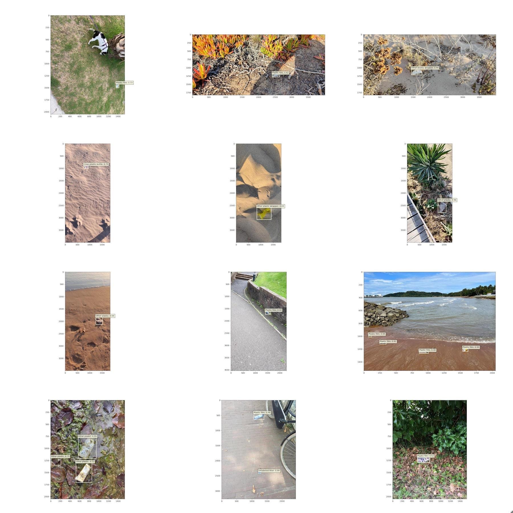
As we can see, our fine tuned model generalizes well to previously unseen images and performs well even in challenging cases of small and blurry objects.
Conclusion
We successfully adapted and fine tuned a pre-trained a Faster R-CNN model on a custom trash detection dataset! We implemented a custom data class and dataloader to handle varying image sizes and annotations, defined a custom model class that leverages a pre-trained model by overwriting the classification head, and wrote a training and validation loop from scratch. We also talked about efficient memory usage and mixed precision training to reduce the memory footprint of the model.
Coding and machine learning aside, environmental pollution is a massive and urgent problem that threatens the whole humanity, and I hope this project inspires you to contribute to the TACO dataset efforts!
We are continuously publishing blog posts with in-depth research reviews and cutting edge code tutorials. To stay up to date with the latest news in AI research, you can follow me on LinkedIn or neuralwork on
Twitter, and LinkedIn.